Color Coordinated Quadrays

Concept by Josef Hasslberger
Execution by Kirby Urner
A work in progress
Version: 0.61
First Posted: October 12, 1997
Last Revised: December 8, 1998


Another game with quadrays involves mapping between quadray coordinates and colors in the Cyan Magenta Yellow Black color specification (CYMK).


CYMK is the four-color standard used in the printing industry, wherein colors reach the eye by light reflecting from paper. On the computer screen, on the other hand, we work with transmitted light using the Red Green Blue standard (RGB).

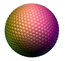
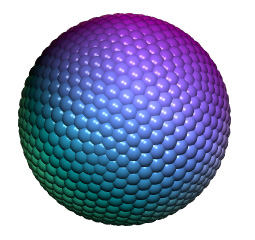
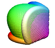
Our goal is to come up with a unit radius sphere whereon each pixel is a of a color determined by its (c,y,m,k) coordinates, translated to RGB for display purposes, and realizing that in each quadrant, one of these primary colors will be set to zero.

quadcolor.gif - 12.5 K


Whereas converting to and from CYMK is a difficult process when true color matching is sought, for mathematical purposes, a mapping to RGB is not that difficult. The above figure shows quadrays from the tetrahedron's center in the four primary colors, with the edges colored using simple linear interpolation, meaning an average of the colors at the two vertices was determined.

The RGB values for the four colors, Cyan, Yellow, Magenta and Black are given below:
cymkrgb.gif - 2.1 K

We compute the average of two primary colors by noticing which of the RGB components change going from one vertex to another, and pick a half way level of 128 for those components. In the chart below, the middle column shows the color obtained by averaging the two primary colors on either side:
midcymk.gif - 3.6 K


The above tetrahedron is only a first approximation to the color sphere we are seeking. Firstly, each edge should actually be a color gradient, with the displayed average color appearing only at the center of the edge, and with the terminal, vertex colors becoming more prominent towards either end. Secondly, each edge should really be an edge of the spherical tetrahedron, such that the radial sweep-out distance from the origin is always constant. All points on the surface within each spherical quadrant will then be a blend of the three primary colors which bound that region.

QUADSPH.gif - 3.7 K


We can develop our spherical tetrahedron CYMK (with color gradient edges) from the six pairings of quadrays. Each of the six arcs will be a vector sum involving just two of the quadrays, such as a and b, with the distance from the origin set at a constant root(6)/2 -- the initial radius of the sphere in which our quadray tetrahedron is inscribed.

The length of a quadray, which may be a vector sum of basis quadrays, is:

distance.gif - 1.7 K


If only two basis quadrays are involved, as in the spherical tetrahedron arc between a and b, then this function reduces to the expression for Arc(a,b) given at right.

Furthermore, if this distance is fixed to give a constant spherical sweepout of radius R, then we can express one vector in terms of the other, e.g. b in terms of a (the reason we have two solutions is examined below).

Since we have fixed R at the value of root(6)/2, the second pair of solutions at right gives us specific values for (0,b,0,0) once (a,0,0,0) has been selected.

ARCDIST.gif - 1.4 K
FIXEDRAD.gif - 1.6 K
CYMKRAD.gif - 1.5 K
BSOLUT.gif - 1.5 K
freehand schematic:
angles not precise


We see at left how the arc subtended by quadrays a and b is carved up into regions. Where a is greater than or equal to 1, b will have two positive solutions, except at one point where the two positive solutions converge. When a is less than 1, b will have only one positive solution.

Clearly a has a maximum allowable value beyond which no vector sum with b will be on the arc. This is the same value, greater than 1, at which the positive solutions for b converge, and where the 2nd root term for both is zero.
This point's address: MAXA.gif - 1.2 K

We are now ready to compute an arc using quadray coordinates. We will generate one set of values by having a range from 1 to root(9/8), giving two values for b, and two points on the arc, for every value of a (or one at the maximum). Then we will let a range from 1 down to 0, taking only the positive solution for b. Repeating this process for all pairs of quadrays will give us our spherical tetrahedron CYMK.


Our strategy for computing data points will center around developing some new methods for cymkTurtle, a subclass of a previously defined '4D turtle' that already knows how to navigate in quadray space. A turtle is a graphical cursor that moves around according to commands. In an object oriented programming language, a turtle contains both methods for executing instructions and storage space for containing specific information, such as current location, distance from the origin, and, in the case of cymkTurtle, CYMK and RGB color values.

A subclass inherits all the methods and data holdings of its parent, while providing a new template capable of accepting additional methods (and/or modifications of old ones) plus data -- all of which may in turn be passed along to future subclasses of turtle in a kind of family tree.

TURTLES.gif - 11.5 K


A core method from cymkTurtle is shown below. A very fine increment is used to move a through its intervals, with a separate calculation placing a right at its maximum value of root(9/8). This last calculation proved necessary for cosmetic reasons: visible nicks appeared in the graphics at these locations even with an increment of 0.005.

    procedure calcarcs
        local a,b1,b2

        * ranging from 1 to root(9/8) by 0.0005
        * grabbing 2 data points
        a=1.0
        do while a<=(9/8)^.5
            b1 = (1/3)*a + (1/3)*(-8*a^2 + 9)^.5
            b2 = (1/3)*a - (1/3)*(-8*a^2 + 9)^.5
            this.runturtle(a,b1)
            if b1<>b2
                this.runturtle(a,b2)
            endif
            a=a+0.0005
        enddo
                
        a  = (9/8)^.5
        b1 = (1/3)*a + (1/3)*(-8*a^2 + 9)^.5
        this.runturtle(a,b1)
        
        * ranging from .999 to 0 by 0.005
        * grabbing 1 data point
        a=0.999
        do while a>=0
            b1 = (1/3)*a + (1/3)*(-8*a^2 + 9)^.5
            this.runturtle(a,b1)
            a=a-0.005
        enddo
    endproc

Complete source code for cymkTurtle is provided as a separate web page, for those interested in all the nitty gritty details -- many of which have to do with the specifics of Visual FoxPro, the computer language used for this implementation (specifics outside the scope of this paper).

BLUETET.gif - 7.3 K


At left is the ray traced output by Povray based on the datapoints table generated by cymkTurtle. The smooth curves of this spherical tetrahedron actually consist of hundreds of tiny partially overlapping spheres each defined by its xyz position and radius (0.04). This interim result confirms that our turtle knows how to generate a spherical tetrahedron.

Since Povray gives us control over the RGB color values for each of the tiny spheres, the next step is to consider how to mix the CYMK primary colors into corresponding mixes of red, green and blue.


An arc between cyan and yellow, for example, involves no change in the RGB value for green, which according to our above chart remains maximized throughout. But in going towards yellow, the value of the red RGB component goes from 0 to 100%, while the blue component drops from 100% to 0. By linking a to cyan and b to yellow, we produce a gradient by means of addition and subtraction.

Below is an excerpt of the cymkTurtle color-calibrating method. It stores RGB values in three columns in our datapoints table, wherein each data point constitutes a row. Note the additional wrinkle: Povray expects its RGB values on a 0 to 1 decimal scale, versus the hexadecimal 0 to 255 scale used in our color charts. This actually makes life easier as our quadray coordinates are likewise in the 0 to 1.06 range -- "close enough for folk music" as the expression goes.

    procedure storecolor(edge,c,y,m,k)
        do case
        
            case edge='ab' && cy
                replace rcolor with 0.0 + y
                replace gcolor with 1.0
                replace bcolor with 1.0 - y

                ... other edges
         endcase
    endproc    

Note that whereas a given CYMK color is purest at its corresponding home vertex, it actually attains a peak value of root(9/8) at three other points, but in mixture with the other colors at the far ends of three respective arcs. This subtle fact is lost in the rounding of RGB color values and produces no visual effect.

Two views of the same colorized spherical tetrahedron are provided below.


QCOLOR0.gif - 8.4 KQCOLOR1.gif - 8.4 K


Over a year after writing the foregoing, I returned to this challenge of generating a colorized CYMK sphere, again using quadray coordinates to control the relative amounts of cyan, magenta, yellow and black. By this time, I had transferred a lot of the features and functionality of my earlier Visual FoxPro routines into a Java application. This new application also had the ability to apply 3-way meshes to the triangular faces of an icosahedron, and inflate these into curved regions.

The graphics below provide two views of a 20-frequency icosaball with the spherical vertices colorized using their quadray coordinates. The procedure is the same as before: the Java utility writes a POV file, which Povray renders as a BMP, which I then resave as a JPEG.

imageimage

The algorithm I used normalizes a generic quadray 4-tuple by dividing through by the largest coordinate. Then I average the RGB contributions of color pairs CY, YM, MB e.g. cyan and yellow each contribute to G (green), so I make G = (C+Y)/2. The K coordinate (black) plays a passive role in that a quadray with a high K value and low C,Y,M values will net an RBG value close to <0,0,0>. Readers might be able to come up with another algorithm that works as well or better.


Additional readings and resources: